CCDC Classification Interface

By Eric Bullock May 7, 2020

Classification of CCDC model parameters for Uganda.

To faciliate easy access to our API we have created a series of graphical user interfaces (GUIs) that require no coding by the user. These guis can be used for calculating CCDC model parameters (i.e. regression coefficients), displaying and interacting with CCDC coefficients and corresponding pixel time series, and classification of the model parameters. This tutorial will demonstrate the gui for creating land cover and land cover change maps.

In this tutorial you will:

• Classify CCDC segments based on their model parameters and ancillary data

• Extract a land cover map for a specific date

• Calculate land cover change between two or more dates

I provide example training data and CCDC coefficients for seven countries in East Africa (Rwanda, Uganda, Ethiopia, Tanzania, Kenya, Zambia, and Malawi).

The first tool that be used in this tutorial can be found here.

1. Classify time series segments

This first step is to classify the time series segments that are the output from the CCDC algorithm. Users should refer to Zhu and Woodcock (2014) for a detailed explanation of the CCDC algorithm. For a refresher, however, the example belows shows the CCDC model fit for the time series of one pixel. On the x-axis is time, and the y-axis is reflectance. Each observation corresponds to a different image at that same location. The parameters of the harmonic regression models, are what we are classifying in this procedure. Thus, we are not classifying Landsat observations, but rather the temporally-continuous model segments. It should be noted that these models are unique for each pixel, and therefore have a unique start and end time depending on land cover or condition change.

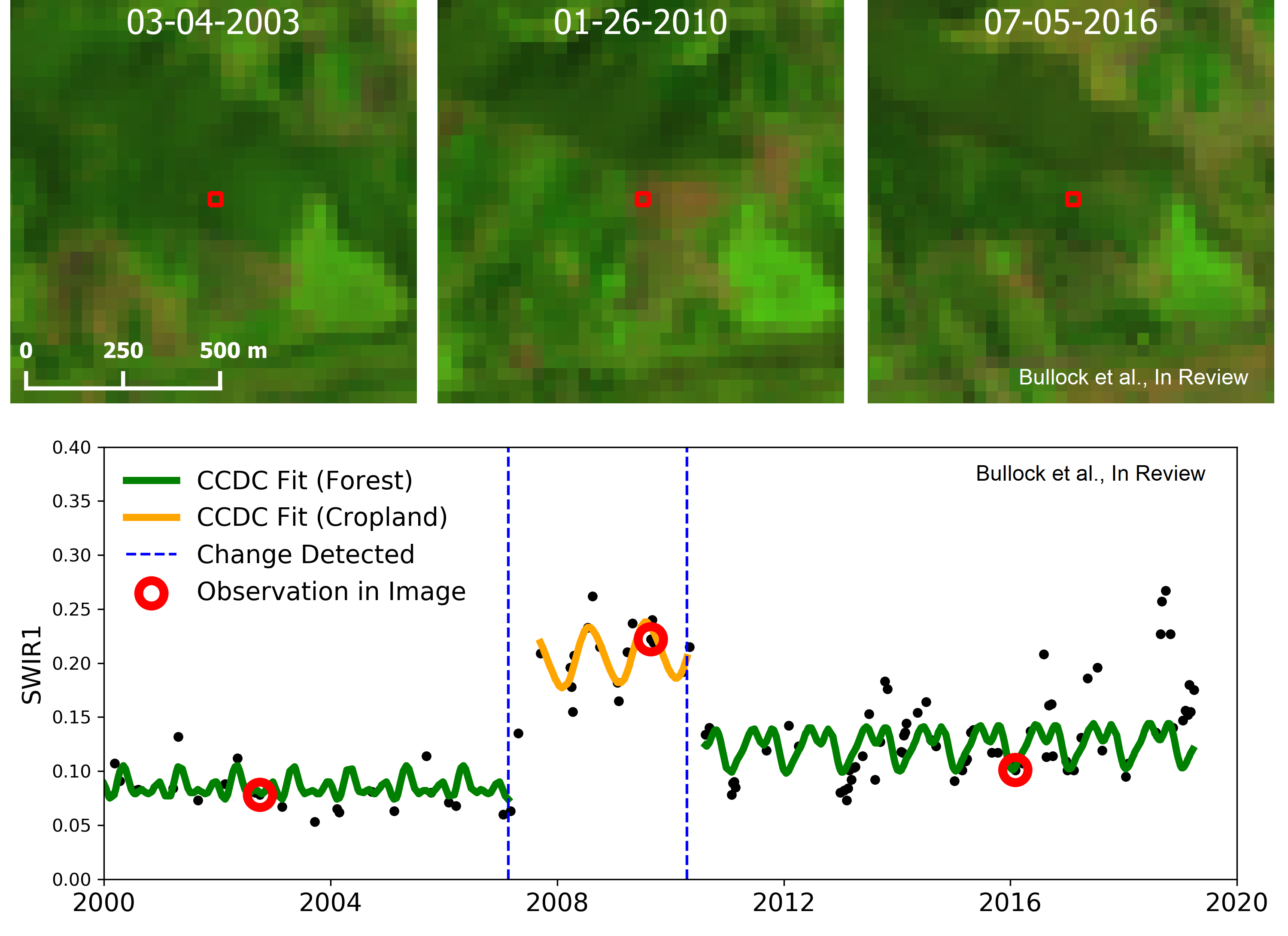
Example CCDC time series for a pixel that is deforested but later return to secondary forest.

This result of part 1 of this tutorial will be an image with bands corresponding to the pixel’s nth land cover label for nbands. In other words, band 1 is the first segment’s classification, band 2 is the second, and so on. Theoretically, a pixel can have dozens of segments. That is very rare, however, since the changes correspond to land change occuring within that pixel. Thus, to reduce computational intensity we limit the number of segments that are classified in this application to 6 per pixel.

The first step is to load the app, you should see a panel like this appear:

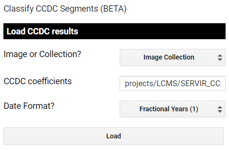
The first step in the app is to load the coefficients.

These first few parameters describe the format of the CCDC results. First, are they saved as a single image or a collection? Next is the path to the CCDC results. In this example, we provide an example of an ImageCollection of results with the path ‘projects/LCMS/SERVIR_CCDC’. Finally, you must specify the date format that the results were run with. For the example dataset they are in the format of ordinal years (0). Click Load.

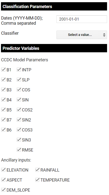
Next comes parameter specification.

Next are the parameters of the machine learning classifier and predictor variables. Uncheck any bands, coefficients, or ancillary data that you do not wish to be used as inputs to classification. The terrain inputs are from the 30m SRTM global DEM, while the climate inputs are from the WorldClim BIO Variables V1.

The next option lets you decide how to define the region to classify and export. As you’ll see, there are many options. Most of them revolve around a global grid that we have created for the Global Land Cover Mapping and Estimation (GLanCE) project. More information on the GLanCE grid grid can be found on the project website.

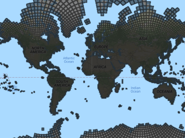
The global GLanCE grid.

There are four ways you can specify a tile to run in addition to manually defining the study region or selecting a country. The simplest option is to choose “Tile Intersecting Point”, and then click somewhere on the map. You will see the grid overlapping the location you selected loaded as the study region.

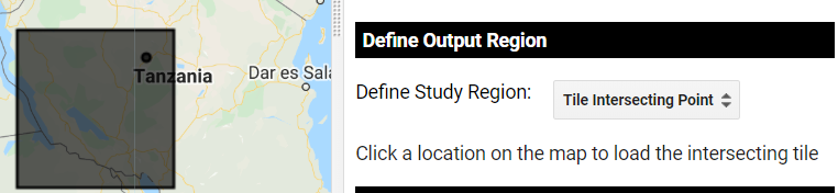
Define study region from the global grid.

Alternatively, you can manually define the study region by clicking on five points on the map that define the borders.

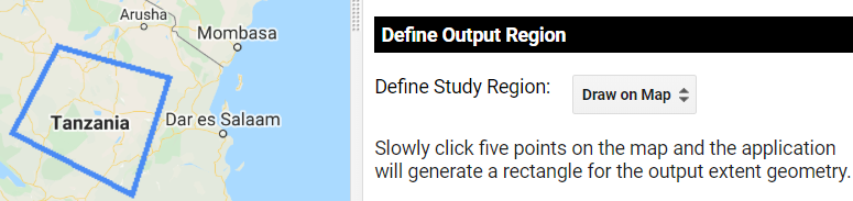
Manually define study region.

The other options are to manually define output grids based on their tile IDs, drawing on the map to specify multiple grids, or selecting a country. If multiple grids are selected then each grid will be submitted as a seperate task. If a country is selected then the entire country boundary will be the study region.

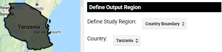
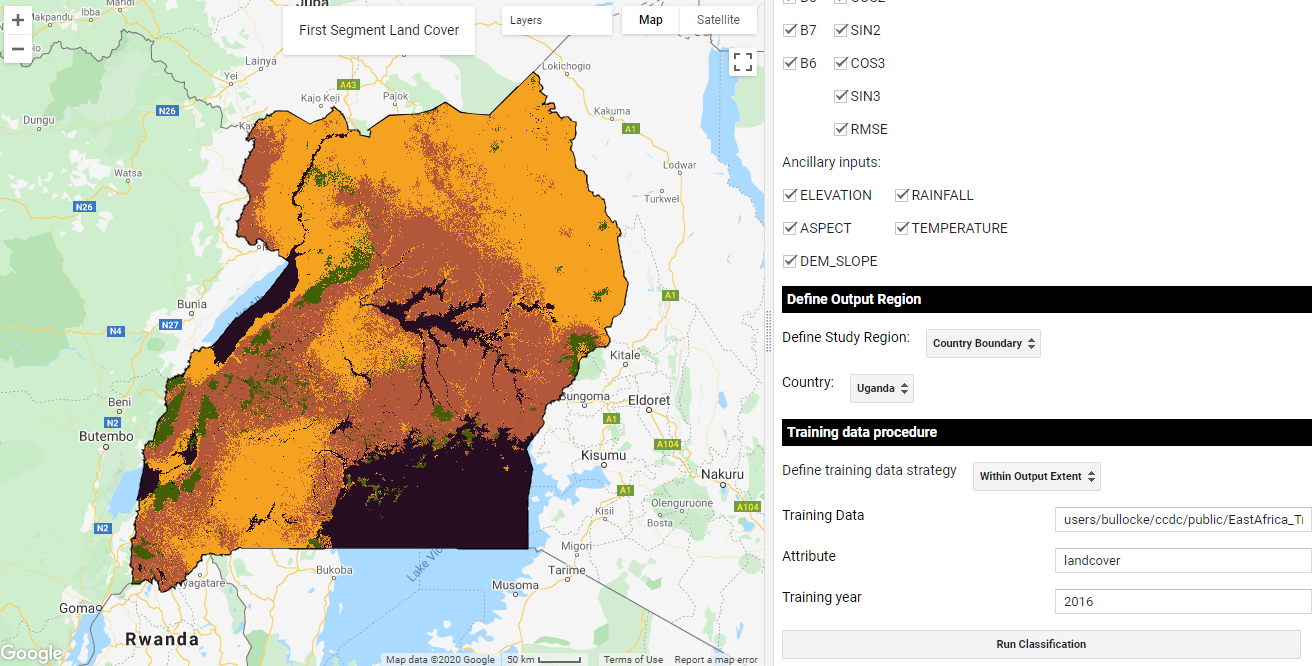
Or an entire country!

The final set of parameters relate to the training data. An example training dataset is provided as a FeatureCollection for the seven countries noted above. The training data requires that each point has an attribute identifying the land cover label, and must also correspond to a specific year for training. You have the option to use the entire FeatureCollection or only the points that fall within the study region.

Classification of the first CCDC segment.

Note, the classification runs quicker if the predictor data for each training point is saved in the feature’s properties (as opposed to being calculated on the fly. I recommend doing this process in a seperate task, and then using the data with the predictors attached to quickly try classification parameters. You should see in the Console a note about whether or not the predictor data must be sampled as the training points. If so, you can also submit a task that will save this calculation for future use.

Finally, when you click ‘Run Classification’, the classification corresponding to the first segment period gets displayed on the map. In this case, the models correspond to ~1999. The full classification stack can be exported as a task that should appear with the description “classification_segments”.

2. Create Land Cover and Land Cover Change Maps

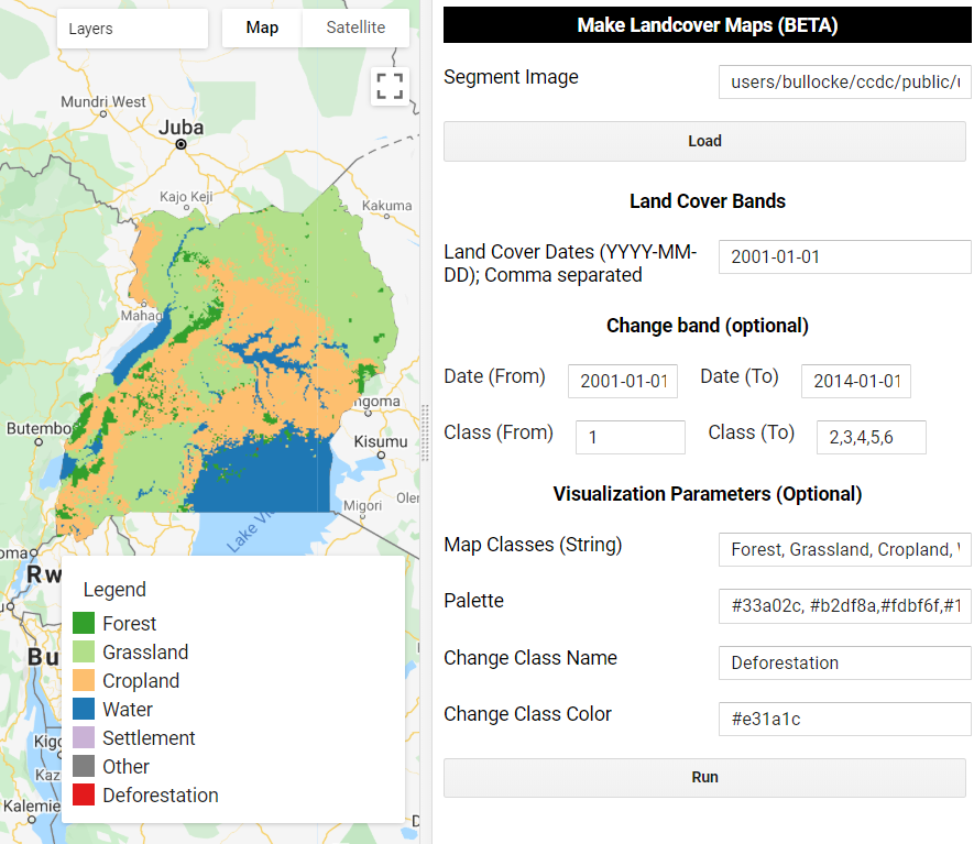
Once the task has completed processing, we can use it to make landcover maps at any date in time for the study region. This asset can be used directly in the Landcover Application. This application is relatively simple - all you need to do is specify the path to the segment image created above and a list of dates and voilà! The dates should be entered in the format ‘YYYY-MM-DD’ and seperated by commas, for example “2001-01-15, 2001-07-21, 2014-12-10”. Each band in the output image will correspond to a different date’s classification.

Land cover classification for 2001-01-01.

This app also has the function to add a change between that represents conversion from one or multiple classes at a specified date to a specified class or group of classes. You must first specify the starting and ending dates and the land cover class # labels for the corresponding dates. For example, the following examples shows the pixels (red) that are class 1 (forest) in 2001-01-01, and are either class 2, 3, 4, or 5 in 2014-01-15. In other words, deforestation from January 2001 to June 2016. You can also specify a single value for the Class (To) box, for example just using 3 would map conversion from 1 to 3, or forest to cropland. If these boxes are left empty then just the land cover maps will be created.

Finally, the tool allows you to specify some visualization parameters. This step is very straightforward, just list the land cover names and corresponding numeric value, and optionally provide a palette.

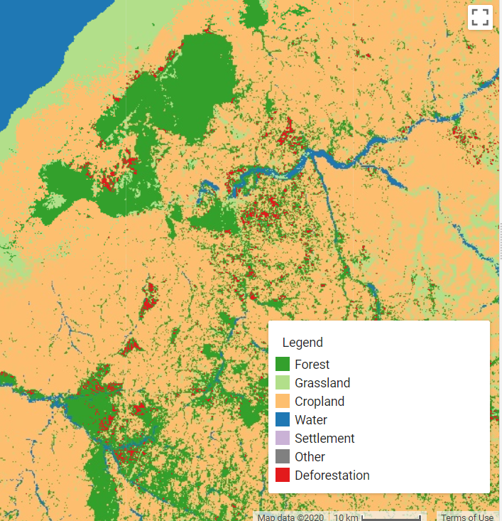
Land cover in 2001 and deforestation between 2001 and 2014.

By default, an opaque hillshade layer is loaded on top of the classification. I find this helps provide context when viewing landscapes that I am unfamiliar with. However, you can simply turn this off in the layers tab.

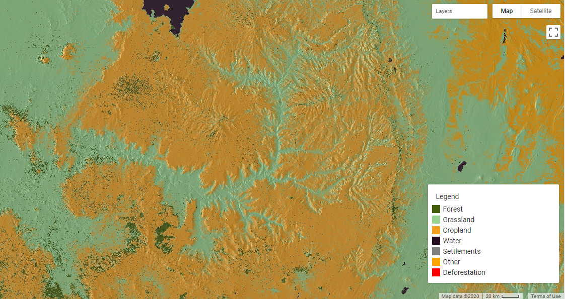
Classified map with a hillshade overlay.