Part 1: Submit Change Detection
Continuous Change Detection and Classification (CCDC) is a land change monitoring that was designed to operate on dense time series of Landsat data. Until recently, use of CCDC has been limited to high-performance computing clusters due to the heavy computation requirements. However, thanks to the outstanding engineers at Google and the US Forest Service, it is now available on the Google Earth Engine (GEE). For a detailed description of the methodology please refer to:
Zhu, Z., & Woodcock, C. E. (2014). Continuous change detection and classification of land cover using all available Landsat data. Remote sensing of Environment, 144, 152-171.
CCDC, as the name implies, has two major components: change detection and classification. This part of the tutorial will focus on the change detection component. Spectral change is detected on a pixel level by testing for structural breaks on the pixel’s time series. In GEE, this process is referred to as ‘temporal segmentation’, as the pixel-level time series are segmented according to periods of unique reflectance. It does so by fitting harmonic regression models to all spectral bands in the time series. The model-fitting starts at the beginning of the time series, and moves forward in time in an “online” approach to change detection. The coefficients are used to predict future observations, and if the residuals of the future observations exceed a statistical boundary for numerous consecutive observations then a change is detected. After the change, a new regression model is fit and the process continues until the end of the time series.
I am not going to go into all of the details of the algorithm, because they are explained in the manuscript above. If this is all new to you, I encourage you to experiment with our CCDC time series viewer app:
https://glance.earthengine.app/view/tstools
Simply navigate to a location (or choose User Location to navigate to your current location), pick a Landsat spectral band, and click on the map to see the CCDC fit to the location you clicked. For example, here is an example of the SWIR1 time series of a location in Rwanda that was forest, converted to cropland, and then converted again to a plantation.
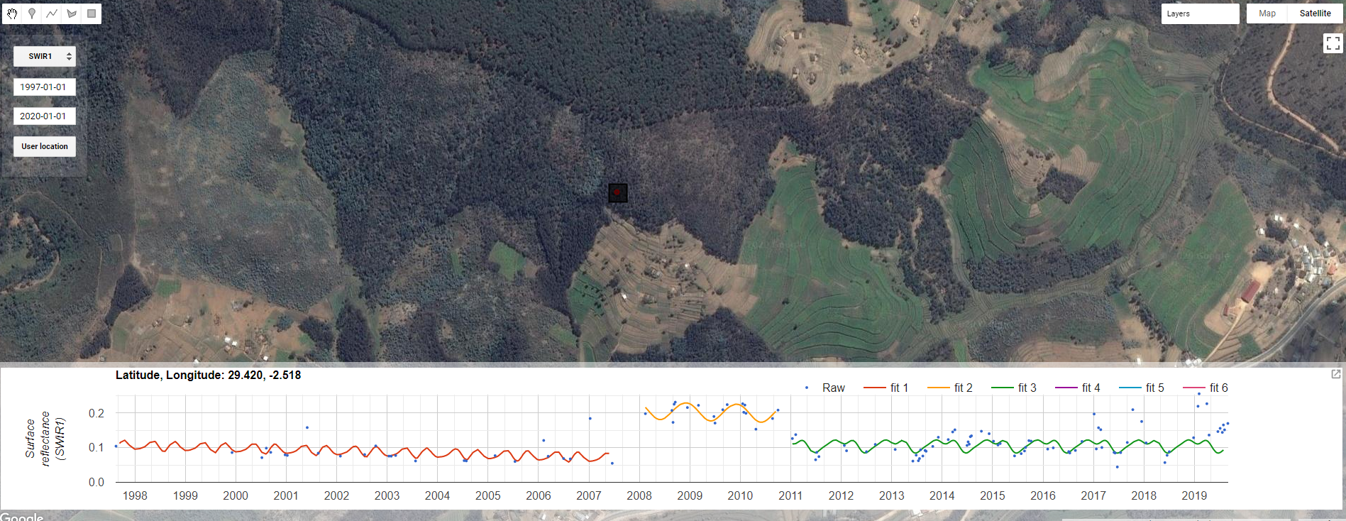
Figure 1. TSTools Earth Engine App
In that example, there were two changes detected: one in 2007 and one in 2010. At this point there are no classification labels associated with the changes, they are simply structural breaks found by the algorithm. This example is for a single pixel, however, and we wish to perform analysis over all the pixels in a study region. This tutorial will demonstrate how to do just that.
CCDC API
To faciliate processing of CCDC mapping on GEE, we have developed an API that contains functions for generating input data, running CCDC, filtering the results, creating “synthetic” Landsat imagery, and classifying the change detection results. The API functions can be found here, and loaded from the following repository:
var utils = require('projects/GLANCE:ccdcUtilities/api')
Building and image stack
The CCDC function in GEE can take any ee.ImageCollection that has been masked for clouds and cloud shadows. CCDC contains an internal cloud masking algorithm and is rather robust against missed clouds, but the cleaner the data the better. If you wish to build your own Image collection, I refer you to the GEE Examples repo. Alternatively, to obtain an image collection of Landsat 4, 5, 7, and 8 data that is masked using the cfmask band you can use the ‘getLandsat’ function in the ‘Inputs’ module of our api. The parameters for building an image collection and running CCDC live within a seperate parameter file
// Load example parameter file
var params = require('projects/GLANCE:Tutorial/params.js')

// Filter by date and a location in Brazil
var filteredLandsat = utils.Inputs.getLandsat()
    .filterBounds(params.StudyRegion)
    .filterDate(params.ChangeDetection.start, params.ChangeDetection.end)

print(filteredLandsat.size())
The console should show that there are around images in the collection. It should be noted that CCDC uses all available Landsat data, even if part of the image is cloudy! That is because there can be many usable, cloud-free pixels even if a majority of the image is cloudy. Since CCDC operates on the pixel time series, those observations are still usable.
Now, we can use this Image Collection into the ee.Algorithms.TemporalSegmentation.Ccdc algorithm and retrieve a multi-dimensional array containing model coefficients, model RMSE, and change information for every detected segment. That means that the dimensions for one pixel can be different than another, depending on the number of model breaks. Documentation on the CCDC parameters are in the GEE Docs, so I will not elaborate on them here.
// First define parameters
var changeParams = {
    collection: filteredLandsat,
    breakpointBands: params.ChangeDetection.breakpointBands,
    tmaskBands: params.ChangeDetection.tmaskBands,
    minObservations: params.ChangeDetection.minObservations,
    chiSquareProbability: params.ChangeDetection.chiSquareProbability,
    minNumOfYearsScaler: params.ChangeDetection.minNumOfYearsScaler,
    dateFormat: params.ChangeDetection.dateFormat,
    lambda: params.ChangeDetection.lambda,
    maxIterations: params.ChangeDetection.maxIterations
  }

var results = ee.Algorithms.TemporalSegmentation.Ccdc(changeParams)
print(results)
And like that, you have run the change detection component of CCDC! A quick note on the output bands:
tStart: The start date of each model segment.
tEnd: The end date of each model segment.
tBreak: The model break date if a change is detected.
numObs: The number of observations used in each model segment.
changeProb: A numeric value representing the multi-band change probability.
*_coefs: The regression coefficients for each of the bands in the image collection.
*_rmse: The model root-mean-square error for each segment and input band.
*_magnitude: For segments with changes detected, this represents the normalized residuals during the change period.
The array can now be saved as an array image. In my experience, array images require the ‘pyramidingPolicy’ to be ‘sample’.
The next part of the tutorial we will go through the process of formatting training data to be used in classification.